Gaussian Beam Propagation: A Recurrence Formula Model for Ideal Lens Systems
table of contents:
-
Gaussian beam shape
First of all, what is a Gaussian beam? A Gaussian beam is a light wave whose intensity distribution is a normal distribution (Gaussian distribution) even in a cross section, such as perpendicular to the direction of light propagation, and laser light is an example of this. It can be represented as shown in the diagram below.

Figure 1-1
Here, each variable is defined as follows:
z: Position in the direction of light travel
w(z): Beam radius at position z
r: distance from the central axis
I(r,z): Light intensity distribution in the r direction at position z
I0 (z): Light intensity on the central axis at position z
In the light intensity distribution I(r,z), the value of r when the light intensity becomes 1/(e^2) times the light intensity I0(z) at the central axis (r=0) is defined as the beam radius w(z) at position z. In this case, I(r,z) can be expressed as follows:

Each parameter is defined below.
λ : wavelength
L: Beam waist position
wo : Beam waist radius
ZR : Rayleigh length θ: divergence angle
Regarding the color coding of each parameter, the amount given by setting is in blue, and the amount given by calculation formula is in black (in the recurrence formula model shown later).
The position where the beam diameter is narrowest is called the beam waist, and the radius of the beam at the beam waist is called the beam waist radius. The beam radius w(z) at position z is expressed as follows using the beam waist position L, beam waist radius w0 , and wavelength λ:

At z = +∞, (1)-② converges to the following.

The inclination of this asymptote is defined as the divergence angle θ.

The distance from the beam waist to the point where the beam diameter expands to √2 times that diameter is called the Rayleigh length, and the distance between them is called the Rayleigh region. This is an important indicator of how far a laser beam can maintain a constant diameter without expanding. The Rayleigh length ZR is expressed as follows:

If we substitute z = L ± ZR into (1)-② and calculate, we can confirm that w(z) = √2 w0 , as defined.
-
Gaussian beam propagation through an ideal lens
Next, consider the propagation of a Gaussian beam through an optical element (assuming the optical element is an ideal lens with no aberrations). The diagram is as follows:
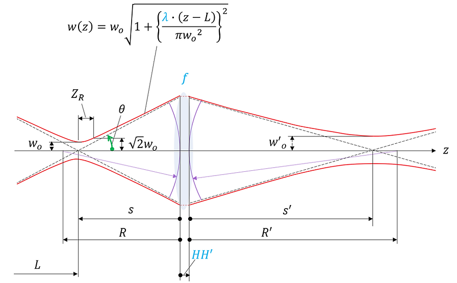
Figure 2-1
*For dimensional notation, see Appendix: Direction and sign of one-dimensional vectors and angles
For each parameter in the above figure, the same ones as those shown in Figure 1-1 are followed, and other new ones are defined as follows.
f : focal length of optical element (ideal lens)
HH' : Distance between principal points of optical elements
R : Radius of curvature of the wavefront just before it enters the optical element
R' : Radius of curvature of the wavefront immediately after it leaves the optical element
s : Distance from the optical element to the beam waist (before passing through the optical element)
s' : distance from the optic to the beam waist (after passing through the optic)
Regarding the color coding of each parameter, the amount given by setting is in blue, and the amount given by calculation formula is in black (in the recurrence formula model shown later) .
The formulas for calculating each parameter are shown below.

From (2)-①b, we can see that the relationship between R and R' has the same form as Gaussian lens formula . In other words, the relationship between the spherical center positions of R and R' is the same as the relationship between the object plane and the image plane in geometric ray tracing. On the other hand, (2)-①c, which shows the relationship between the beam waist positions s and s', is similar to Gaussian lens formula but has a slightly different form. This is a correction of the geometric model Gaussian lens formula that takes into account the effects of light diffraction, and is a formula proposed by Sidney Self et al. in 1983 [1] .
from (2)-①c:

The relationship between s/f and s' / f can be illustrated using ZR / f as a parameter as follows:

Figure 2-2
ZR / f = 0 represents the same state as Gauss's imaging formula in geometric optics. At this point, s' / f diverges to ±∞ when s / f = -1. As the value of Z R / f increases, s' / f begins to take on finite upper and lower limits, and when s / f = -1, s' / f = 0. As the value of ZR / f increases further, the range of possible values for s' / f narrows. This means that the distance the beam waist can travel through a lens is finite, and to maximize this distance, the Rayleigh length (before propagation), ZR , must be as short as possible, and the focal length, f , must be as long as possible .
-
Recurrence formula model for Gaussian beam propagation in an ideal lens system
Next, consider a recurrence model of beam propagation when a Gaussian beam passes through an array of optical elements (assuming the optical elements are ideal lenses with no aberrations). The diagram is as follows:

Figure 3-1
*For dimensional notation, see Appendix: Direction and sign of one-dimensional vectors and angles
Here, the subscript i of each parameter represents the physical quantity related to the i-th optical element from the beam incident position. For each parameter, the amount given by setting is in blue, and the amount given by calculation is in black.
For each parameter in the above figure, the same ones as those shown in Figure 1-1 and Figure 2-1 are followed, and other new ones are defined below.
di : Distance from the i-th optical element to the (i+1)-th optical element
The formulas for calculating each parameter for the i-th optical element are shown below.
・Adding the subscript i to each parameter in (1)-①, it will look like this:

・Adding the subscript i to each parameter in (2)-①, it will look like this:

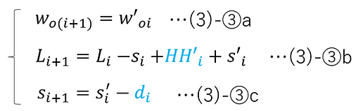
Next, the recurrence formula that holds between the i-th optical element and the (i+1)-th optical element is as follows:
In Figure 3-1, the beam diameter is depicted as the same immediately before and after it enters the optical element, because that is what actually happens. This will be explained below.
The beam diameters just before and just after entering the i-th optical element can be calculated as follows:


Therefore, it was shown that the beam diameter is equal immediately before and after it enters the i-th optical element.
Next, we will show the first term of the recurrence formula. The diagram below shows it.

Figure 3-2
Here too, for each parameter, the amount given by setting is in blue, and the amount given by the calculation formula is in black.
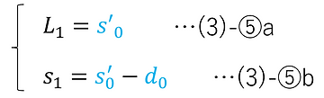
As shown in the figure above, the first term wo1 of woi is given as a set value. Also, the first term L1 of Li and the first term s1 of si are expressed as follows using the set values s'0 and d0 :
-
Recursive formula model for real Gaussian beam propagation in an ideal lens system
(3)-①a shows that the product of woi and θi is a constant that does not depend on i. This is defined as BPP (Beam Parameter Product).

Furthermore, if the beam radius of the actual beam is woi_real and the beam divergence angle of the actual beam is θi_real , the product of woi_real and θi_real is also a constant that does not depend on i. This is defined as BPPreal .

By taking the ratio of (4)-①a to (4)-①b, we can obtain M2 (M-squared), a quantity that represents the beam quality shown below. Since neither (4)-①a nor (4)-①b depends on i, M2 is also a quantity that does not depend on i. This means that if there is no influence of aberrations in the optical elements, the value of M2 can be obtained by actually measuring the beam radius and beam divergence angle for any single i.

The value of M2 is 1 or more, and the closer the value is to 1, the closer it is to an ideal Gaussian beam.
Here, we assume that the actual beam is spread while maintaining a normal (Gaussian) distribution compared to an ideal Gaussian beam, and M2 represents the degree of this spread. Therefore, it should be noted that this approximation is not sufficient for beams where the normal distribution itself is significantly deviated from.
Similar to the ideal Gaussian beam in the previous chapter, we will consider the actual beam propagation when a Gaussian beam passes through a series of optical elements (ideal lenses). Here, the actual measurement of the beam is performed before it enters the optical system (i.e., at the first term of the recurrence formula). The diagram is as follows:

Figure 4-1
*For dimensional notation, see Appendix: Direction and sign of one-dimensional vectors and angles
Here, the subscript i of each parameter represents the physical quantity related to the i-th optical element from the beam incidence position. Also, for each parameter, the amount given by setting is in blue, and the amount given by calculation is in black. Also, since all calculated quantities (except M2) have values that differ from those of an ideal Gaussian beam, the subscript "real" is used to distinguish them.
The definitions of each parameter in the above figure follow those shown in Figures 1-1, 2-1, and 3-1.
The formulas for calculating each parameter for the i-th optical element are shown below.
・Adding the subscript "real" to each parameter in black in (3)-①, it will look like this:

・Adding the subscript "real" to each parameter in black in (3)-②, it will look like this:

Similarly, the recurrence formula that holds between the i-th optical element and the (i+1)-th optical element is as follows, according to (3)-③.

Next, we will show the first term of the recurrence formula. The diagram below shows it.

Figure 4-2
Here too, for each parameter, the amount given by setting is in blue, and the amount given by the calculation formula is in black.
There are several cases for what to set as the first term of the recurrence formula, but here, the first term wo1_real of woi_real and the first term θ1_real of θi_real are given as set values. These are given by actual measurements, or in the case of fiber input, the mode field diameter of the fiber corresponds to 2 x wo1_real. The conditions for the first term can be illustrated as follows:
In this case, M2 is given by:

The first term L1_real of Li_real and the first term s1_real of si_real are expressed as follows using the setting values s'0 and d0 .

-
Excel calculation format
Using the calculation model explained so far, we have created an Excel simulation format that actually simulates the propagation of a Gaussian beam. Please feel free to use it.
・Gaussian beam propagation (ideal)
・Gaussian beam propagation (real)
-
References
-
Related literature
[A] Kishikawa, Toshiro. Yūzā Enjinia no Tame no Kōgaku Nyūmon (An Introduction to Optics for User Engineers). Optronics Co.
-
Update History
-
2025-11 Completely revised
-
2025-07 Newly released