Geometrical ray propagation in ideal lens systems based on lens formula

First, we derive the equation for the imaging relationship. Then, we show a recurrence model of geometric ray propagation through an ideal lens, applying Newton's Formula. We also show how to construct an imaging optical system by specifying the initial value of the ray and automatically calculating the final value.

This shows the results of ray tracing of an imaging optical system with an ideal lens (focal length: f). The method is to apply Newton's formula (or Newton's relation) to the recurrence formula.

*The content explained here is only a model of geometrical optics ray propagation, and does not take into account the effects of wave optics diffraction. For Gaussian beam propagation, the effects of wave optics diffraction must be taken into account, and the theoretical model is different, so please refer to the link below.

Recurrence formula model for Gaussian beam propagation through ideal lenses

・Derivation of the imaging relationship formula

The manner in which a ray of light from an object point passes through an optical element with a focal length f and is focused onto an image point is illustrated below.

*For dimensional notation, see Appendix: Direction and sign of one-dimensional vectors and angles

(i) When f > 0, z < 0,

This diagram shows how a ray of light from an object point passes through an ideal lens with focal length f to form an image. Newton's formula can be found from this diagram.

(ii) When f > 0, 0 < z < f,

Ray tracing with ideal lens arrangement_002.png

(iii) When f > 0, f < z,

Ray tracing with ideal lens arrangement_003.png

(iv) When f < 0, z < f

Ray tracing with ideal lens arrangement_004.png

(v) When f < 0, f < z < 0,

Ray tracing with ideal lens arrangement_005.png

(vi) When f < 0, z > 0 ,

Ray tracing with ideal lens arrangement_006.png

If the magnification is β, then due to the similarity of triangles, the following can be said for all of (i) to (vi).

Next, consider the following:

From the figure, the following can be said:

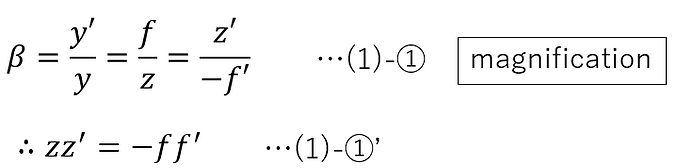
From (1)-①', (1)-②a, and (1)-②b,

From Lagrange invariant,

From (1)-④, (1)-②abc, and (1)-①',

From (1)-① and (1)-⑤,

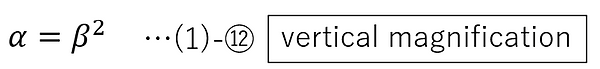
Next, if we define the longitudinal magnification α as follows, then from (1)-①, (1)-①', and (1)-⑥,

It should be noted that this only holds true when z is a small quantity.

*When the medium is air:

Since n=n'=1, the following can be said.

From (1)-①, (1)-①', and (1)-⑧, we obtain the following equations, including Newton's equations (or Newton's relations).

ガウスの結像式

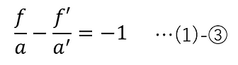
Next, by applying (1)-(3) to (1)-(8), the following Gaussian imaging formula is obtained.

Next, the object-to-image distance will be described.
If the object-image distance is defined as a one-dimensional vector with the object point as the start point and the image point as the end point, it can be expressed as follows:

縦倍率

Next, for the vertical magnification, by substituting n=n'=1 into (1)-⑦, the following formula is obtained.

・Recurrence formula model for geometric ray propagation through ideal lenses

I consider a method of arranging ideal lenses in order and tracing rays using Newton's formula.

First, the settings required for ray tracing are as follows:

Settings for side 0:

・Object height: h0

・Angle of the light ray coming out of the object: θ0

・Distance from the object surface to the front principal point of the first optical element: d0

Settings for page i：

・Focal length of optical element: fi , (f'i )

・Distance between principal points of optical elements: HH'i

・Distance from the rear principal point to the front principal point of the next surface: di

The diagram for the 0th and 1st surfaces is as follows:

*For dimensional notation, see Appendix: Direction and sign of one-dimentional vectors and angles

Ray tracing with ideal lens arrangement_025.png

However, the settings are in blue and the values calculated from the recurrence formula are in black.

The conditions shown in the figure can be expressed as the following equations.

Ray tracing with ideal lens arrangement_045.png

Here, the medium is air and (1)-⑧ is applied.
In addition, θ0 and θ1 are assumed to be minute amounts.
In this case, if we rearrange (2)-①, we get the following:

Ray tracing with ideal lens arrangement_027.png

Next, the i-th and (i+1)-th faces are illustrated below.

*For dimensional notation, see Appendix: Direction and sign of one-dimentional vectors and angles

Ray tracing with ideal lens arrangement_046.png

However, the settings are in blue and the values calculated from the recurrence formula are in black.

The conditions shown in the figure can be expressed as the following equations.

Ray tracing with ideal lens arrangement_047.png

Here, the medium is air and (1)-⑧ is applied.
Also, θi and θi+1 are assumed to be minute amounts.
In this case, (2)-③ can be rearranged as follows:

Ray tracing with ideal lens arrangement_030.png

Therefore, by inputting values for the settings of each surface and performing calculations (2)-② and (2)-④ in order from the 0th surface to the nth surface (image surface), ray tracing can be performed.

・Setting the initial state of the light

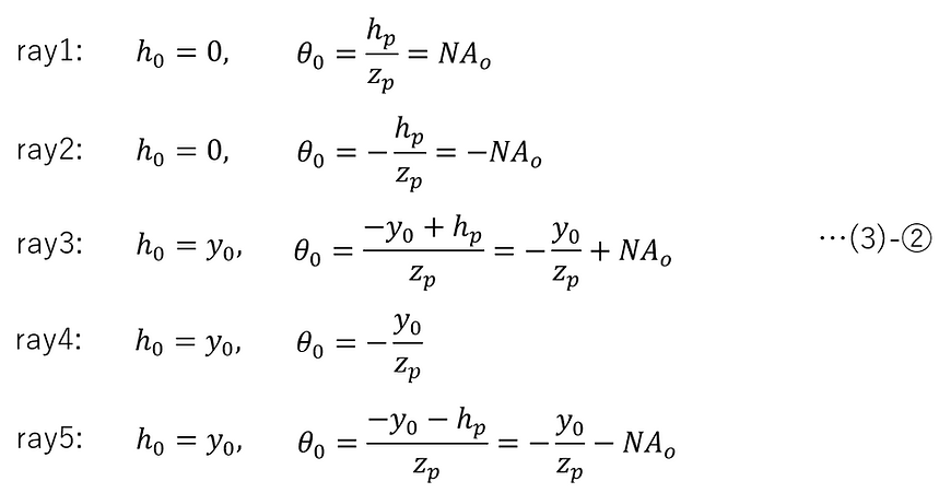
Next, let us consider how to set the setting values h0 and θ0 for the 0th surface .
There are various possible methods, but here it is given by the entrance pupil position and the object side numerical aperture.

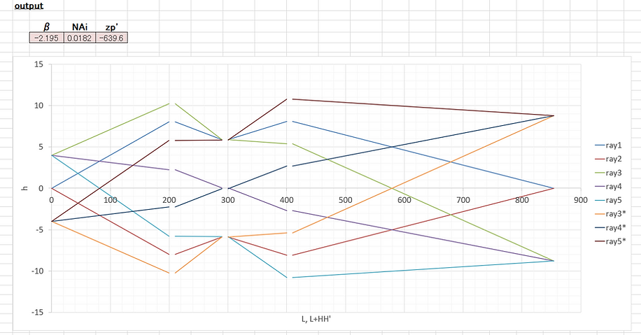
By setting the object height y0 , the distance to the entrance pupil zp , and the object-side numerical aperture NAo, we can obtain the five light rays (ray1, ray2, ..., ray5) shown in the figure below.

Ray tracing with ideal lens arrangement_072.png

Here, D is the entrance pupil diameter. If the angle φ is assumed to be infinitesimal, NAo can be expressed as follows:

Ray tracing with ideal lens arrangement_069.png

Therefore, the setting values h0 and θ0 of the 0th surface, which represent each of the rays ray1, ray2, ..., ray5, can be calculated as follows.

Ray tracing with ideal lens arrangement_071.png

・Calculating the closing value of a ray

Finally, the parameters of the optical system and image plane are automatically calculated.

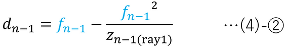
For ray1 (or ray2), calculate dn-1 so that the position where the ray intersects with the central axis after passing through the optical element at the (n-1)-th surface becomes the image surface (the n-th surface) .

In this case, if the light ray for ray1 from the (n-1)-th surface to the n-th surface (image surface) is illustrated, it will look like this:

Ray tracing with ideal lens arrangement_118.png

The conditions shown in the figure for ray1 can be expressed as follows.

Ray tracing with ideal lens arrangement_112.png

Here, if we assume that the medium is air and apply (1)-⑧, we get the following:

Ray tracing with ideal lens arrangement_113.png

Then, by using the ray height hn(ray3) of ray3 at the image plane position , the magnification β of the entire optical system can be found by calculating the following:

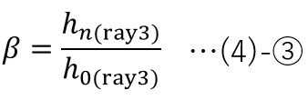
Ray tracing with ideal lens arrangement_110.png

Furthermore, the image-side numerical aperture NAi can be calculated as follows:

Ray tracing with ideal lens arrangement_083.png

For ray 4, the position where the ray intersects with the central axis after passing through the optical element at the (n-1)-th surface is the exit pupil position. The distance from the rear principal point of the (n-1)-th surface to the exit pupil is denoted by dn-1(p) , and the distance from the image plane to the exit pupil is denoted by zp'.

In this case, if the light ray 4 from the (n-1)-th surface to the exit pupil surface is illustrated, it will look like this:

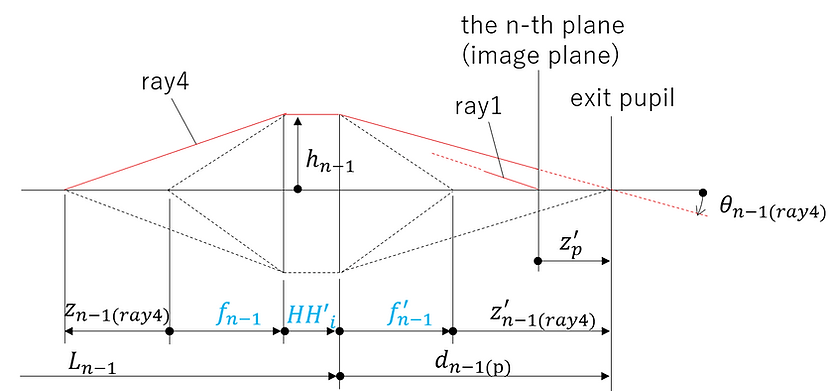
Ray tracing with ideal lens arrangement_119.png

The conditions shown in the figure for ray4 can be expressed as follows.

Ray tracing with ideal lens arrangement_107.png

Here, if we assume that the medium is air and apply (1)-⑧, we get the following:

Ray tracing with ideal lens arrangement_108.png

Therefore, the exit pupil position zp' can be calculated as follows.

Ray tracing with ideal lens arrangement_114.png

・Creating a format for ray tracing

We will now show an example of how to apply the recurrence formula shown above to create a format in Excel for arranging an ideal lens and tracing rays.

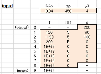
・Input section:

Enter the values for each setting item in the black box below. There are up to 9 surfaces, but it is not necessary to enter all of them. For the remaining surfaces, the focal length should be set to a sufficiently large value equivalent to infinity, and the principal point distance and surface distance should be set to zero.

Ray tracing with ideal lens arrangement_101.png

・Calculation section:

Ray tracing calculations are performed separately for each of rays 1 to 5. The red and blue boxes refer to the input values.

Ray tracing with ideal lens arrangement_100.png

・Ray tracing data section:

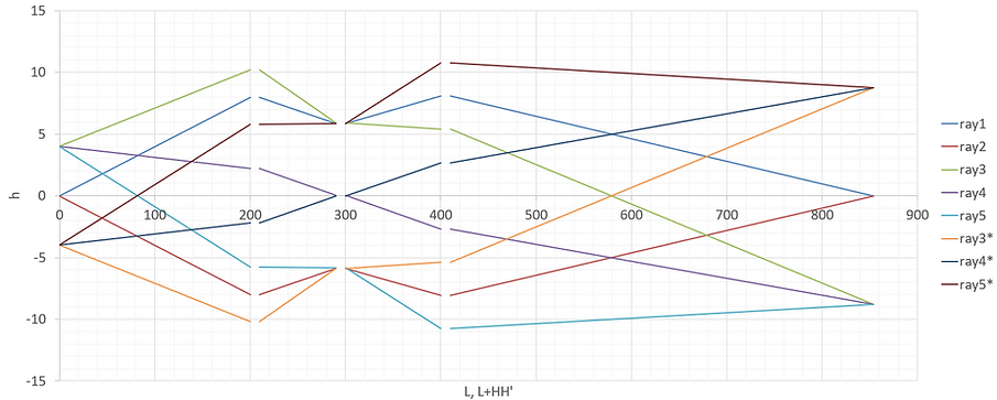
The following is data for plotting the results of ray tracing. The position in the optical axis direction is given for each surface as L and L+HH'. Also, lines are left blank to avoid drawing rays between principal points. For rays 3, 4, and 5, new rays 3*, 4*, and 5* have been added, which are inverted with respect to the optical axis.

Ray tracing with ideal lens arrangement_099.png

・Ray tracing result display section:

The results of the ray tracing are shown in the figure below. The calculation results of the optical system and image plane parameters are also shown.

Ray tracing with ideal lens arrangement_098.png

In this way, you can use Excel to place an ideal lens and perform ray tracing. The format is shown below.