Paraxial ray propagation in a spherical lens system and the Lagrange invariant
A ray in the paraxial region has a very small angle θ with respect to the optical axis of the optical system, and all of its paths pass very close to the optical axis. In this case, the following approximation holds for θ:
sin θ = θ, tan θ = θ, cos θ = 1
Therefore, limiting the area to the paraxial region makes ray tracing calculations extremely simple and is useful for understanding the structure of the optical system. Here, we will show how to derive the calculation formula.
table of contents:
・Derivation of Abbe's invariants
When a ray of light passes through the boundary surface (spherical shape) of a material, the ray of light in the paraxial region can be illustrated as follows:
(i) When u > 0, u' > 0,

Figure 1-1
(ii) When u > 0, u' < 0,

Figure 1-2
*For dimensional notation, refer to Appendix: Definitions of direction and sign for one‑dimensional vectors and angles
The parameters in the above figure are defined as follows:
n : Refractive index of the material before incidence on the boundary surface
n' : Refractive index of the material after exiting the boundary surface
r : Radius of curvature of the boundary surface
u: The angle between the incident ray on the boundary surface and the central axis (counterclockwise is positive)
u': Angle between the exit ray from the boundary surface and the central axis (counterclockwise is positive)
i: The angle between the incident light on the boundary surface and the normal to the boundary surface (counterclockwise is positive)
i': The angle between the light emitted from the boundary surface and the normal to the boundary surface (counterclockwise is positive)
φ: The angle between the normal at the incident position of the ray on the boundary surface and the central axis (counterclockwise is positive)
h: Height of the ray at the boundary surface relative to the central axis
s: The distance from the boundary surface to the point where the incident light intersects with the central axis
s': Distance from the boundary surface to the point where the light emitted from the boundary surface intersects with the central axis
Here, the angles u , u' , φ , i , i' and the height h are assumed to be sufficiently small. Also, the color coding for each parameter is as follows: the amount given by the setting is in blue, and the amount given by the calculation formula is in black (in the recurrence formula model shown later).
In this case, the conditions shown in the figure can be expressed as the following equations in both (i) and (ii).

Here, the fact that both (i) and (ii) are expressed by the same equation means that they are both forms of the same model, and it can be said that it is sufficient to consider either one of them.
From (1)-①abc, the following is derived.

Furthermore, according to Snell's law , the following can be said in the paraxial region:
From (1)-①'ab and (1)-②, the Abbe's invariant shown below can be derived.

(1)-③ (Abbe's invariant) describes a ray traveling from point P to point P', and it can be seen that u, u', and h are not included in it. From this, it can be said that in the paraxial region, as shown in Figure 1-3, any ray passing through point P travels toward point P' (i.e., points P and P' are conjugate).

Figure 1-2
・Derivation of Lagrange invariant
When the entire system is rotated around point O (the center of the sphere on the boundary surface), point P moves to point Q and point P' moves to point Q'. Points Q and Q' are also conjugate, but since the boundary surface remains completely unchanged before and after rotating the entire system, it can be said that points Q and Q' were also conjugate before rotating the entire system.
Here, in the paraxial region, arcs PQ and P'Q' can be considered as straight lines perpendicular to the central axis, so the vectors PQ and P'Q' can be treated as vectors perpendicular to the central axis.

Figure 2-1
For each parameter, those shown in Figures 1-1 and 1-2 will be followed, and new parameters will be defined as follows.
y: object height
y': image height
ω: Angle of the ray from the object height y toward the intersection of the boundary surface and the optical axis
ω': Angle of the ray from the intersection of the boundary surface and the optical axis toward image height y'
In this case, the conditions shown in the figure can be expressed as the following equations:

Furthermore, according to Snell's law, the following can be said in the paraxial region:
From (1)-①a, (2)-①ab, and (2)-②, the following relationship can be obtained.

This relation is called the Lagrange invariant or the Helmholtz-Lagrange invariant.
・Recurrence relations and matrix notation for paraxial calculations
Consider a system in which a ray passes through the 0th surface (object surface), the 1st surface, the 2nd surface, ..., the j-th surface, ..., and the k-th surface (image surface) in that order. Here, each surface is assumed to be spherical (flat surfaces are given with an infinite radius of curvature). In this case, if we illustrate the ray in the paraxial region before and after passing through the j-th surface, it looks like this:

Figure 3-1
*For dimensional notation, refer to Appendix: Definitions of direction and sign for one‑dimensional vectors and angles
The subscript j of each parameter means the j-th boundary surface.
For each parameter in the above diagram, those shown in Figures 1-1 and 1-2 will be retained, and new ones will be defined as follows.
dj : Distance from the j-th surface to the (j+1)-th surface
Here again, we assume that the angles uj , u'j , and height hj are sufficiently small. Also, for each parameter, the values given by the settings are shown in blue, and the values given by the calculation formula are shown in black .
First, from (1)-①a, the following can be said about the j-th plane.

Furthermore, from (1)-③ (Abbe's invariant), the following can also be said for the j-th plane.

From (3)-①,②,

Furthermore, the following can be said from Figure 3-1.
Here, we set it as follows:

Applying this to (3)-②',③ yields the following equation.

(3)-⑤a,b can be represented as matrices as follows, which allows for efficient calculation of the recurrence relation.

(3)-⑥ Combining a and b results in the following:

Next, from (2)-③ (Lagrange invariants), the j-th plane is as follows:

From Figure 3-1, we have n'j = nj+1 , u'j = uj+1 , and y'j = yj+1 , so we can also say the following.
From (3)-⑦,⑧, the following can be said.

・Deriving optical system parameters through paraxial calculations
Here, the initial conditions and output values are given for the following two cases.
(i) In the case of parallel light incidence
In this case, as shown in the figure below, the initial condition of the recurrence formula (exiting the object surface) and the terminal condition of the recurrence formula (exiting the k-th surface) are given, and the focal length f is obtained as the output value of the optical system parameter.

From (1)-①a,

Therefore, dk can be calculated as follows:

Also, from the figure, the focal length f can be calculated as follows:

Here, in the case of parallel light incidence, d0 does not affect subsequent calculations. Also, in the definition of the paraxial region, h0 is an infinitesimal quantity, but the calculation of the focal length does not depend on the value of h0 (not just on infinitesimal quantities) .
(ii) In the case of a finite system
In this case, as shown in the figure below, the initial condition of the recurrence formula (exiting the object surface) and the terminal condition of the recurrence formula (exiting the k-th surface) are given, and the magnification β is obtained as the output value of the optical system parameter.

From (1)-①a,

Therefore, dk can be calculated as follows:

From (3)-⑨ (the recurrence relation for Lagrange's invariants), the multiplier β can be calculated as follows.
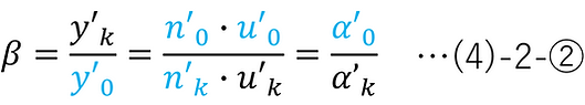
Here, in the definition of the paraxial region, u'0 is an infinitesimal quantity, but the calculation of the magnification does not depend on the value of u'0 (not just on infinitesimal quantities).
The calculation format based on what has been explained so far is shown below.
・Specific example: Formula for calculating the focal length of a single lens (Lens-Maker's formula)
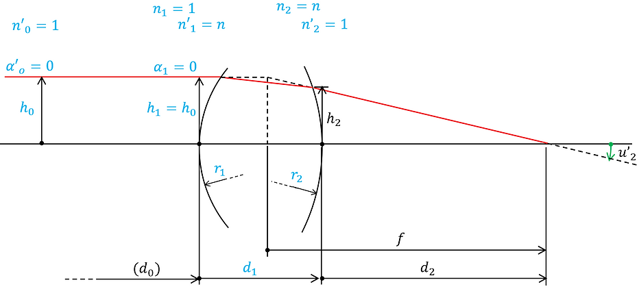
Here, we will derive the formula for calculating the focal length of a single lens from the paraxial calculation formula. If we apply the refractive index of the material, n, the radius of curvature of the first and second surfaces, r1 and r2, respectively, and the center thickness, d1, to the paraxial calculation model, we get the figure below.
First, we obtain the following paraxial calculation formula from (3)-⑥a,b and (3)-⑥'.

Furthermore, from (4)-1-①,②, the following can be obtained.

Applying the parameter values in the figure (h1=h0 , n1=n'2=1, n'1 =n2=n, α1=0) to (5)-① gives the following:

From (5)-②ab, (5)-③, and n'2 =1 in the figure, the following is obtained.

The obtained (5)-②b' is called the Lens-Maker's Formula.
-
Related literature
[A] Kishikawa, Toshiro. Yūzā Enjinia no Tame no Kōgaku Nyūmon (An Introduction to Optics for User Engineers). Optronics Co.
-
Update History
-
2026-04: The flow of the first half has been significantly reorganized.
-
2025-10: Newly released