Coherence Length of Optical Waves: A Theoretical Model Derived from Spectral Shape
Here, we will derive the relationship between the coherence length of a light wave and the spectral width of a light source for the following two cases.
<1> When the light source spectrum is a normal distribution
Here, the depth resolution in OCT (Optical Coherence Tomography) generally uses the value derived from the model in <1>, which will also be shown in the latter half of <1>. It is important to note that in OCT, the light reflected from the object being measured is detected, resulting in a round-trip path, and the depth resolution is half the value of the coherence length.
<1> When the light source spectrum is a normal distribution
Step 1: Derive the spectral width in k-space
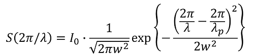
The spectral characteristics of a light wave are expressed as a normal distribution (Gaussian distribution) in k-space (wave number space) as follows:

where I0 is the total intensity of the light wave, kp is the wavenumber at which S(k) peaks, and w is the standard deviation of the spectrum in k-space.
The diagram of S(k) is as follows:

Here, the following definitions are made:
・The wave number at which S(k) is half the peak is kH.
・The half-width of the spectrum in k-space is Δk.
In this case,

Therefore,
Step 2: Derive the spectral width in λ space
In ①, k=2π / λ, k p = 2π / λ p Then, when converted to λ space (wavelength space),
S(2π/λ) can be illustrated as follows:

Here, the following definitions are made:
・λ H± is the wavelength when S(2π/λ) is half the peak
・Δλ is the full width at half maximum of S(2π/λ)
In this case,
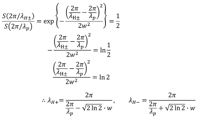
Therefore,

Step 3: Derive the coherence length in real space
Let E(x) be the distribution of light waves in real space (x space).
Furthermore, the position where the amplitude reaches its peak is denoted by x p , and the phase at the position x p is denoted by −δ.
In this case,

Here, the following is obvious (from the properties of odd functions).

Therefore,

Here, the following is set:

From the interchange of integrals and derivatives theorem [1], we can say the following.

Solving this equation gives us the following:


Where:

Therefore,

Therefore,

E(x) can be illustrated as follows:

Here, the following definitions are made:
・E A± (x) is the amplitude of E(x)
・x H± is the position when E A± (x) is halfway to the peak
・Δx is the full width at half maximum of E A± (x)
In this case,

Therefore,

Step 4: Derive the relationship between Δx and Δλ
From ② and ③, we finally obtain the following relationship.

*The value of the coefficient 0.88 on the right-hand side changes slightly depending on how Δx and Δλ are defined.
The relationship between Δx and Δλ can be illustrated as follows:

Application: Relationship between OCT depth resolution and coherence length
The depth resolution in OCT (Optical Coherence Tomography) generally uses a value derived from equation ④ obtained using a model in which the light source spectrum is normally distributed, so here we will show the relationship between OCT depth resolution and coherence length.As shown in the figure below, when observing light reflected from an observation surface in a material with a refractive index of n, we consider the relationship between depth resolution Δd and coherence length Δx.

The coherence length Δx calculated so far is the distance in air, so the distance in a material must be considered in terms of the air-equivalent length. Also, when observing reflected light, the optical path length is twice the actual distance, since it is the round-trip distance. Taking this into consideration, the relationship between coherence length and depth resolution is as follows:


<2> When limiting the bandwidth of a wide spectral light source with a bandpass filter (i.e., a step-shaped spectrum )
Step 1: Derive the spectral width in k-space
The spectral characteristics of a light wave are expressed as a step-shaped distribution in k-space (wave number space) as follows:
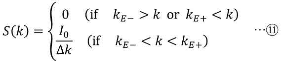
however,

where I0 is the total intensity of the light wave, kp is the wavenumber in the middle of the spectral band in k-space, kE± are the wavenumbers at the edges of the spectral band, and Δk is the width of the spectral band.
S(k) can be illustrated as follows:

Step 2: Derive the spectral width in λ space
In ⑪, k=2π/λ, k E±=2π/λE̠∓, converting to λ space (wavelength space), we get the following:
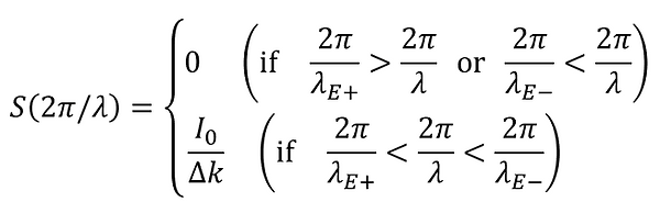
however,

Furthermore, put it as follows:

In this case, the relationship between Δλ and Δk is derived as follows:

Therefore, S(2π/λ) is as follows:

S(2π/λ) can be illustrated as follows:

Step 3: Derive the coherence length in real space
Let E(x) be the distribution of light waves in real space (x space).
Also, the position where the amplitude reaches its peak is defined as xp, and the phase at the position xp is defined as −δ.
At this time,

E(x) can be illustrated as follows:

where EA± (x) is the amplitude of E(x).
In this case, the coherence length can be defined in the following two ways.
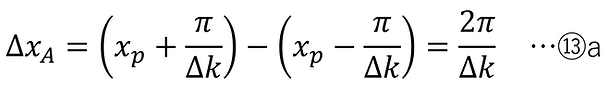
(i) When half the full width of the main lobe is defined as the coherence length ΔxA
EA+(x) becomes zero at ±2π/Δk relative to xp ( the width between these zero points is the full width of the main lobe). At half that , ±π/Δk, EA+(x) becomes 2/π times the peak , and the width 2π/Δk at this time is defined as the coherence length ΔxA .
(ii) When the full width at half maximum of the main lobe is defined as the coherence length ΔxB
ΔxB can be calculated as follows:

This is difficult to solve analytically, so we can calculate it numerically as follows:

Step 4: Derive the relationship between Δx and Δλ
(i) When the coherence length is defined as ΔxA
From ⑫ and ⑬a,

(ii) When the coherence length is defined as ΔxB
From ⑫ and ⑬b,

・References
・Related literature
[A] Goodman, JW “Statistical Optics.” Wiley (1985 / 2000).
[B] Born & Wolf, “Principles of Optics.” Cambridge University Press.
[C] Mandel & Wolf, “Optical Coherence and Quantum Optics.” Cambridge UP.
-
Update History
-
2025-11: Added "<2> When limiting the bandwidth of a wide spectral light source with a bandpass filter (i.e., a step-shaped spectrum )"
-
2025-09: Added "Application: Relationship between OCT depth resolution and coherence length".
-
2025-04: Newly released